Diffusion models explained
An overview of diffusion models (work in progress).
Introduction
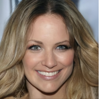
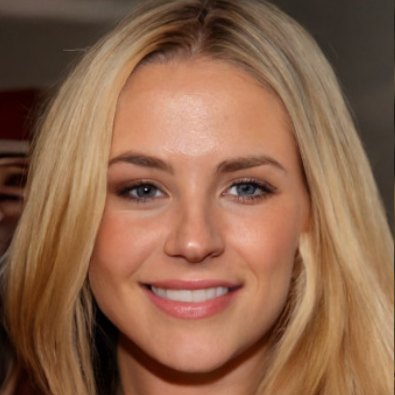
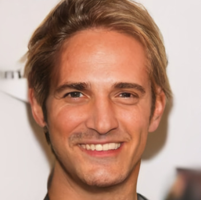
If you are reading this post, then you may have heard that diffusion models are kind of the big thing for generating high-quality image data. Simply see below:

However, grasping diffusion models may seem initially daunting, and you may easily get confused by terms such as denoising diffusion and score-based generative models. Therefore, this blog post aims to provide a big picture of diffusion models, whether you prefer to call them diffusion, denoising diffusion, or score-based diffusion models. All of them have the same roots, the diffusion process, so I will refer to them as Diffusion models and make it explicit when a singular idea comes from a particular approach.
For more in-depth information, I will always suggest reading the original papers:
I also recommend reading the following blog post, from which some information I have added here to provide a complete picture.
Before starting, I would like to recall that modeling high-dimensional distributions where training, sampling, and evaluating probabilities are tractable is not easy. As a result, approximation techniques such as variational inference and sampling methods have been developed over the years. Now, with Diffusion models, we can do that and more!
Diffusion models
Diffusion Models are probabilistic models that are capable of modeling high-dimensional distributions using two diffusion processes: 1) a forward diffusion process maps data to a noise distribution, i.e., an isotropic Gaussian, and 2) a reverse diffusion process that moves samples from the noise distribution back to the data distribution. The essential idea in diffusion models, inspired by nonequilibrium statistical physics and introduced by Sohl-Dickstein et al.
Stochastic processes are sequences of random variables that can be either time-continuous or discrete. Because a diffusion process is a stochastic process, diffusion models can be time-continuous or discrete. Therefore, I will start first by explaining time-discrete diffusion models. Once we have grasped the fundamental idea, we will move to time-continuous diffusion processes, which generalize the time-discrete diffusion process where an Itô stochastic differential equation describes the evolution of the system.
Discrete diffusion models
Notation
It may be helpful to keep in mind this standard notation when using discrete diffusion models.
- \( q_0(\mathbf{x}_0) \): the unknown data distribution
- \( p_{\theta}(\mathbf{x}_0) \): the model probability
- \( q(\mathbf{x}_0, ... , \mathbf{x}_T) \): the forward trajectory (chose by design)
- \( p_{\theta}(\mathbf{x}_0, ..., \mathbf{x}_T) \): the parametric reverse trajectory (learnable)
Lets assume that our dataset consists of \( N \) i.i.d inputs \( \{\mathbf{x}_0^n\}_{n=0}^N \sim q_0(\mathbf{x}) \) sampled from an unknown distribution \( q_0(\mathbf{x}_0) \), where the lower-index is used to denoted the time-dependency in the diffusion process. The goal is to find a parametric model \( p_{\theta}(\mathbf{x}_0) \approx q_0(\mathbf{x}_0) \) using a reversible diffusion process that evolves over a discrete time variable \( t \in[0,T] \).
Forward process
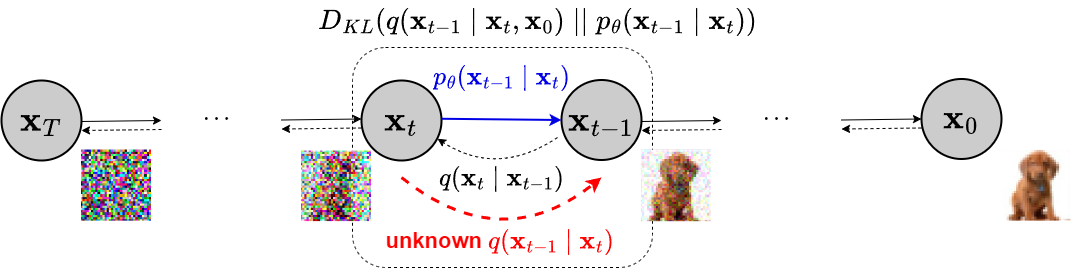
The forward diffusion process, represented by a Markov chain, is a sequence of random variables \( (\mathbf{x}_{0}, \dots, \mathbf{x}_{T}) \) where \( \mathbf{x}_0 \) is the input data (initial state) with probability density/distribution \( q(\mathbf{x}_0) \) and the final state \( \mathbf{x}_T\sim \pi(\mathbf{x}_T) \), where \( \pi(\mathbf{x}_T) \) is an easy to sample distribution, i.e., an Isotropic Gaussian. Each transition in the chain is governed by a perturbation kernel \( q(\mathbf{x}_t \vert \mathbf{x}_{t-1}) \). The full forward trajectory, starting from \( \mathbf{x}_0 \) and performing \( T \) steps of diffusion, due to the Markov property, is:
$$ q(\mathbf{x}_{0:T})= q(\mathbf{x}_0) \prod_{t=1}^T q(\mathbf{x}_t \vert \mathbf{x}_{t-1} ) $$
Figure 2 shows, with dotted lines (from right to left), how the forward diffusion process systematically perturbed the input data $\mathbf{x}_0$ over time $t\in[0,T]$ using $q(\mathbf{x}_t \vert \mathbf{x}_{t-1})$, gradually converting $\mathbf{x}_0$ into noise, losing slowly its distinguishable features as $t$, the diffusion step, becomes larger. Eventually, when $T \to \infty$, $\mathbf{x}_T$ is equivalent to an isotropic Gaussian distribution. The stationary distribution is chosen by design, so the forward process does not have learnable parameters. Sohl-Dickstein et. al.
$$ \begin{equation} \label{eq:transition_kernel} q(\mathbf{x}_t \vert \mathbf{x}_{t-1}) = \mathcal{N}(\mathbf{x}_t; \sqrt{1 - \beta_t} \mathbf{x}_{t-1}, \beta_t\mathbf{I}) \end{equation} $$
where \( \beta_t \) is the variance schedule, a sequence of positive noise scales such that \( 0 < \beta_1, \beta_2, ..., \beta_T < 1 \). This model in the literature is also known as DDPM
A nice property of the above process is that we can sample \( \mathbf{x}_t \) at any arbitrary time step $t$ in a closed form using reparameterization trick. Let \( \alpha_t = 1 - \beta_t \) and \( \bar{\alpha}_t = \prod_{i=1}^t \alpha_i \), and now \( q(\mathbf{x}_t \vert \mathbf{x}_{t-1}) = \mathcal{N}(\mathbf{x}_t; \sqrt{\alpha_t} \mathbf{x}_{t-1}, 1-\alpha_t\mathbf{I}) \)
$$ \begin{aligned} \mathbf{x}_1 &= \sqrt{\alpha_1}\mathbf{x}_0 + \sqrt{1 - \alpha_1}\mathbf{\epsilon}_0 \quad\quad\quad\quad\quad\text{ ;where } \mathbf{\epsilon}_0, \mathbf{\epsilon}_1, \dots \sim \mathcal{N}(\mathbf{0}, \mathbf{I}) \\ \mathbf{x}_2 &= \sqrt{\alpha_2}\mathbf{x}_1 + \sqrt{1 - \alpha_2}\mathbf{\epsilon}_1\\ &= \sqrt{\alpha_2}\left(\sqrt{\alpha_1}\mathbf{x}_0 + \sqrt{1 - \alpha_1}\mathbf{\epsilon}_0\right) + \sqrt{1 - \alpha_2}\mathbf{\epsilon}_1\\ &= \sqrt{\alpha_2\alpha_1}\mathbf{x}_0 + \underbrace{\sqrt{\alpha_2(1 - \alpha_1)}\mathbf{\epsilon}_0}_{\mathbf{\epsilon}_0^*} + \underbrace{\sqrt{1 - \alpha_2}\mathbf{\epsilon}_1}_{\mathbf{\epsilon}_1^*}\\ &= \sqrt{\alpha_2\alpha_1} \mathbf{x}_0 + \sqrt{1 - \alpha_1\alpha_2}\bar{\mathbf{\epsilon}}_1 \quad\quad\quad\text{ ;where } \bar{\mathbf{\epsilon}}_{1} \text{ merges two Gaussians (*).} \\ &= \dots \\ x_t &= \sqrt{\bar{\alpha}_t}\mathbf{x}_0 + \sqrt{1 - \bar{\alpha}_t}\mathbf{\epsilon}_{t} \\ q(\mathbf{x}_t \vert \mathbf{x}_0) &= \mathcal{N}(\mathbf{x}_t; \sqrt{\bar{\alpha}_t} \mathbf{x}_0, (1 - \bar{\alpha}_t)\mathbf{I}) \quad\quad\quad\text{ ; Transition density function.} \end{aligned} $$
(*) Recall the properties of the sum of two Gaussian random variables. Let \( \mathbf{\epsilon}_0^* \sim \mathcal{N}(\mathbf{\mu}_0, \sigma^2_0\mathbf{I}) \), and \( \mathbf{\epsilon}_1^{*} \sim \mathcal{N}(\mathbf{\mu}_1, \sigma^2_1\mathbf{I}) \). Then, the new random variable \( \mathbf{z}= \mathbf{\epsilon}_0^*+ \mathbf{\epsilon}_1^* \) has density \( \mathcal{N}(\mathbf{\mu}_0+\mathbf{\mu}_1, (\sigma^2_0+\sigma^2_1)\mathbf{I}) \). First we can de-reparametrized \( \epsilon_0^* \) and \( \epsilon_1^* \) so we get \( \mathcal{N}(0,Var(\epsilon_0^*)) \) and \( \mathcal{N}(0,Var(\epsilon_1^*)) \) correspondingly. We have that the sum of these two Gaussians is
$$ \begin{aligned} \mathbf{z}&= \mathbf{\epsilon}_{0}^{*}+ \mathbf{\epsilon}_{1}^{*}\\ &=\mathcal{N}(0,Var(\epsilon_0^{*})+ Var(\epsilon_1^{*}))\\ &=\mathcal{N}(0,(1 - \alpha_1 \alpha_2)\mathbf{I}))\quad\quad\quad \text{ ;Using the property of the variance (*).}\\ &=\sqrt{1- \alpha_1 \alpha_2}\bar{\mathbf{\epsilon}}_{1} \quad \text{ ;where } \bar{\mathbf{\epsilon}}_{1}\sim \mathcal{N}(\mathbf{0}, \mathbf{I}) \text{ and used reparameterization}\\ \end{aligned} $$
(*) Recall that \( Var(aX) = a^2 Var(X) \); Therefore, we have the following
\( Var(\epsilon_0^*) = Var(\sqrt{\alpha_2(1 - \alpha_1)}\mathbf{\epsilon}_0)= \alpha_2(1 - \alpha_1) \)
\( Var(\epsilon_1^*) =Var(\sqrt{1 - \alpha_2}\mathbf{\epsilon}_1)= 1 - \alpha_2 \)
\( Var(\epsilon_0^*) + Var(\epsilon_1^*)= \alpha_2(1 - \alpha_1)1 - \alpha_2= 1 - \alpha_1 \alpha_2 \)
More concretely, we can sample $\mathbf{x}_t$ for any timestep $t$ in closed form given $\mathbf{x}_0$ using the so-called t-step transition probability.
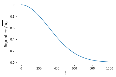
$$ \begin{equation} \label{eq:transition_t} q(\mathbf{x}_t \vert \mathbf{x}_0) = \mathcal{N}(\mathbf{x}_t; \sqrt{\bar{\alpha}_t} \mathbf{x}_0, (1 - \bar{\alpha}_t)\mathbf{I}) \end{equation} $$
where \( \bar{\alpha}_t \) is an decreasing function such that \( \bar{\alpha}_1 < ... < \bar{\alpha}_T \). The power signal of \( \mathbf{x}_0 \) decreases over time while the noise intensifies. Figure 3 shows a 2D animation of the behavior of the forward diffusion process where each transition is governed by equation \ref{eq:transition_t} for 4 different inputs \( \mathbf{x}_0 \) located at (10,-10), (-10,-10), (10,10), and (10,-10). Each input trajectory is repeated three times to observe the stochastic behavior of the diffusion process. The forward diffusion process will systematically move all \( \mathbf{x}_0 \)'s to an Isotropic Gaussian distribution as \( t\rightarrow T=1000 \).

In summary: the forward diffusion process maps any sample to a chosen stationary distribution. For this example, under the transition kernel of equation \ref{eq:transition_t}, to an Isotropic Gaussian.
- The forward process \( \mathcal{F} \) has a structure that allows us to observe meaningful evolution over time and ensures that this is tractable, given the Markov property.
Reverse process
If we know how to reverse the forward process and sample from \( q(\mathbf{x}_{t-1} | \mathbf{x}_t) \), we will be able to remove the added noise, moving the Gaussian distribution back to the data distribution \( q(\mathbf{x}_0) \). For this, we learn a parametric model \(p_{\theta}(\mathbf{x}_{0:T})\) to approximate these conditional probabilities to run the reverse process.
$$ \begin{equation} \label{eq:reverse_trajectory} p_\theta(\mathbf{x}_{0:T}) = p(\mathbf{x}_T) \prod^T_{t=1} p_\theta(\mathbf{x}_{t-1} | \mathbf{x}_t) \quad p_\theta(\mathbf{x}_{t-1} | \mathbf{x}_t) = \mathcal{N}(\mathbf{x}_{t-1}; \mathbf{\mu}_\theta(\mathbf{x}_t, t), \mathbf{\Sigma}_\theta(\mathbf{x}_t, t)) \end{equation} $$
This reverse process is similarly define by a Markov chain with learned Gaussian transitions starting at \( p(\mathbf{x}_T)= \mathcal{N}(\mathbf{x}_T;\mathbf{0}, \mathbf{I}) \). The reversal of the diffusion process has the identical functional form as the forward process as \( \beta \rightarrow 0\)
Then a generative Markov chain converts \( q_T \approx p_{\theta}(\mathbf{x}_T) \), the simple distribution, into a target (data) distribution using a diffusion process. Figure 2. shows how the generative Markov chain generates samples like the training distribution starting from \( \mathbf{x}_T \sim p(\mathbf{x}_T) \). The model probability is defined by:
$$ \begin{equation} p_{\theta}(\mathbf{x}_0) = \int p_{\theta}(\mathbf{x}_{0:T}) dx_{1:T} \end{equation} $$
This integral is intractable. However, using annealed importance sampling and the Jarzynski equality we have:
$$ \begin{aligned} p_{\theta}(\mathbf{x}_0) &= \int p_{\theta}(\mathbf{x}_{0:T}) {\color{blue}\frac{q(\mathbf{x}_{1:T}| \mathbf{x}_0)}{q(\mathbf{x}_{1:T}\vert \mathbf{x}_0)}} dx_{1:T}\\ &= \int q(\mathbf{x}_{1:T} | \mathbf{x}_0) \frac{p_{\theta}(\mathbf{x}_{0:T})}{q(\mathbf{x}_{1:T}\vert \mathbf{x}_0)} dx_{1:T}\\ &= \int q(\mathbf{x}_{1:T} | \mathbf{x}_0) p(\mathbf{x}_T) \prod^T_{t=1} \frac{p_\theta(\mathbf{x}_{t-1} | \mathbf{x}_t)}{q(\mathbf{x}_t | \mathbf{x}_{t-1})} dx_{1:T}\\ &= \mathbb{E}_{q(x_{1:T} | x_0)}\left[p(x_T) \prod_{t=1}^T \frac{ p(x_{t-1}|x_t)}{q(x_t|x_{t-1})}\right] \end{aligned} $$
\( q(\mathbf{x}_{0:T}) = q(\mathbf{x}_{1:T} | \mathbf{x}_0)q(\mathbf{x}_0) \rightarrow q(\mathbf{x}_{1:T} | x_0) = \frac{q(\mathbf{x}_{0:T})}{q(\mathbf{x}_0)} = \frac{q(\mathbf{x}_0) \prod_{t=1}^T q(\mathbf{x}_t | \mathbf{x}_{t-1})}{q(\mathbf{x}_0)} =\prod_{t=1}^T q(\mathbf{x}_t | \mathbf{x}_{t-1}) \) The model probability is, therefore, the relative likelihood of the forward and reverse trajectories averaged over forward trajectories \( q(\mathbf{x}_{1:T} | \mathbf{x}_0) \). This objective function can be efficiently evaluated using only a single sample from \( q(\mathbf{x}_{1:T} | \mathbf{x}_0) \) when the forward and reverse trajectories are identical (when \( \beta \) is infinitesimally small). This form corresponds to the case of a quasi-static process in statistical physics.
For infinitesimal $\beta$ the forward and reverse distribution over trajectories can be made identical
Training
We train by minimizing the cross entropy (CE) \( H \left[q(\mathbf{x}_0), p_{\theta}(\mathbf{x}_0) \right] \) between the true underlaying distribution \( q(\mathbf{x}_0) \) and the model probability \( p_{\theta}(\mathbf{x}_0) \)
$$ \begin{aligned} L_\text{CE} &= \mathbb{E}_{q(\mathbf{x}_0)}\left[ -\log p_\theta(\mathbf{x}_0) \right] \\ &= \mathbb{E}_{q(\mathbf{x}_0)}\left[ -\log \Big( \mathbb{E}_{q(\mathbf{x}_{1:T} | \mathbf{x}_0)} \left[ p(\mathbf{x}_T) \prod^T_{t=1} \frac{p_\theta(\mathbf{x}_{t-1} | \mathbf{x}_t)}{q(\mathbf{x}_t\vert \mathbf{x}_{t-1})} \right] \Big)\right] \\ &\leq \mathbb{E}_{q(\mathbf{x}_0)}\left[ \mathbb{E}_{q(\mathbf{x}_{1:T} \vert \mathbf{x}_0)} \left[-\log \Big(p(\mathbf{x}_T) \prod^T_{t=1} \frac{p_\theta(\mathbf{x}_{t-1} \vert \mathbf{x}_t)}{q(\mathbf{x}_t\vert \mathbf{x}_{t-1})}\Big)\right] \right] \\ &\leq \mathbb{E}_{q(\mathbf{x}_{0:T})} \left[-\log \Big(p(\mathbf{x}_T) \prod^T_{t=1} \frac{p_\theta(\mathbf{x}_{t-1} \vert \mathbf{x}_t)}{q(\mathbf{x}_t | \mathbf{x}_{t-1})}\Big) \right] \\ &= \mathbb{E}_{q(\mathbf{x}_{0:T})}\Big[\log \frac{q(\mathbf{x}_{1:T} | \mathbf{x}_{0})}{p_\theta(\mathbf{x}_{0:T})} \Big] = L_{\text{VLB}}\\ &= \mathbb{E}_{q(\mathbf{x}_{0:T})} \left[-\log p(\mathbf{x}_T) - \log\prod^T_{t=1} \frac{p_\theta(\mathbf{x}_{t-1} \vert \mathbf{x}_t)}{q(\mathbf{x}_t\vert \mathbf{x}_{t-1})} \right] \\ &= \mathbb{E}_{q(\mathbf{x}_{0:T})} \left[-\log p(\mathbf{x}_T) - \sum^T_{t=1}\log \frac{p_\theta(\mathbf{x}_{t-1} \vert \mathbf{x}_t)}{q(\mathbf{x}_t\vert \mathbf{x}_{t-1})} \right]\\ &= L_{\text{VLB}_\text{simplify}} \end{aligned} $$
We use Jensen's inequality \( \mathbb{E}[f(x)] \ge f(\mathbb{E}[x]) \) for convex function. Making use of the fact that \(-\log(x) \) is convex we have that \( \mathbb{E}[-\log(x)] \ge -\log(\mathbb{E}[x]) \). Further improvements come from variance reduction by rewriting the equation as:
$$ \begin{aligned} L_\text{VLB} &= \mathbb{E}_{q(\mathbf{x}_{0:T})}\Big[\log \frac{q(\mathbf{x}_{1:T} \vert \mathbf{x}_{0})}{p_\theta(\mathbf{x}_{0:T})} \Big]\\ &= \mathbb{E}_{q(\mathbf{x}_{0:T})} \left[-\log p(\mathbf{x}_T) - \sum^T_{t=1}\log \frac{p_\theta(\mathbf{x}_{t-1} \vert \mathbf{x}_t)}{q(\mathbf{x}_t\vert \mathbf{x}_{t-1})} \right]\\ &= \mathbb{E}_{q(\mathbf{x}_{0:T})} \left[-\log p(\mathbf{x}_T) - \sum^T_{t=2}\log \frac{p_\theta(\mathbf{x}_{t-1} \vert \mathbf{x}_t)}{q(\mathbf{x}_t\vert \mathbf{x}_{t-1})} - \log \frac{p_\theta(\mathbf{x}_0 \vert \mathbf{x}_1)}{q(\mathbf{x}_1\vert \mathbf{x}_0)} \right]\\ &= \mathbb{E}_{q(\mathbf{x}_{0:T})} \left[-\log p(\mathbf{x}_T) - \sum^T_{t=2}\log \frac{p_\theta(\mathbf{x}_{t-1} \vert \mathbf{x}_t)}{q(\mathbf{x}_{t-1} \vert \mathbf{x}_t, \mathbf{x}_0)}\cdot\frac{q(\mathbf{x}_{t-1} \vert \mathbf{x}_0)}{q(\mathbf{x}_t \vert \mathbf{x}_0)} - \log \frac{p_\theta(\mathbf{x}_0 \vert \mathbf{x}_1)}{q(\mathbf{x}_1\vert \mathbf{x}_0)} \right];\quad \text{Markov property + Bayes' rule (*).}\\ &= \mathbb{E}_{q(\mathbf{x}_{0:T})} \left[-\log p(\mathbf{x}_T) - \sum^T_{t=2}\log \frac{p_\theta(\mathbf{x}_{t-1} \vert \mathbf{x}_t)}{q(\mathbf{x}_{t-1} \vert \mathbf{x}_t, \mathbf{x}_0)} - \sum^T_{t=2}\log\frac{q(\mathbf{x}_{t-1} \vert \mathbf{x}_0)}{q(\mathbf{x}_t \vert \mathbf{x}_0)} - \log \frac{p_\theta(\mathbf{x}_0 \vert \mathbf{x}_1)}{q(\mathbf{x}_1\vert \mathbf{x}_0)} \right] \\ &= \mathbb{E}_{q(\mathbf{x}_{0:T})} \left[-\log p(\mathbf{x}_T) - \sum^T_{t=2}\log \frac{p_\theta(\mathbf{x}_{t-1} \vert \mathbf{x}_t)}{q(\mathbf{x}_{t-1} \vert \mathbf{x}_t, \mathbf{x}_0)} - \log\frac{\color{blue}q(\mathbf{x}_1 \vert \mathbf{x}_0)}{q(\mathbf{x}_T \vert \mathbf{x}_0)} - \log \frac{p_\theta(\mathbf{x}_0 \vert \mathbf{x}_1)}{\color{blue}q(\mathbf{x}_1\vert \mathbf{x}_0)} \right] \quad \text{Suming up (**).}\\ &= \mathbb{E}_{q(\mathbf{x}_0)}\left[ \mathbb{E}_{q(\mathbf{x}_{1:T} \vert \mathbf{x}_0)} \left[ \log\frac{q(\mathbf{x}_T \vert \mathbf{x}_0)}{p(\mathbf{x}_T)} - \sum^T_{t=2}\log \frac{p_\theta(\mathbf{x}_{t-1} \vert \mathbf{x}_t)}{q(\mathbf{x}_{t-1} \vert \mathbf{x}_t, \mathbf{x}_0)} - \log p_\theta(\mathbf{x}_0 \vert \mathbf{x}_1) \right]\right]\\ &= \mathbb{E}_{q(\mathbf{x}_0)}\left[ \text{D}_{KL}(q(\mathbf{x}_T \vert \mathbf{x}_0)||p(\mathbf{x}_T)) + \sum^T_{t=2} \text{D}_{KL} (q(\mathbf{x}_{t-1} \vert \mathbf{x}_t, \mathbf{x}_0)||p_\theta(\mathbf{x}_{t-1} \vert \mathbf{x}_t)) - \log p_\theta(\mathbf{x}_0 \vert \mathbf{x}_1) \right] \end{aligned} $$
(*) Because of the Markov property of the diffusion process \( q(\mathbf{x}_t \vert \mathbf{x}_{t-1})= q(\mathbf{x}_t \vert \mathbf{x}_{t-1}, \mathbf{x}_0) \).
(*) Using Bayes' rule
$$ \begin{align} \label{eq:forward_posterior} q(\mathbf{x}_{t-1} \vert \mathbf{x}_t, \mathbf{x}_0) = \frac{q(\mathbf{x}_t \vert \mathbf{x}_{t-1}, \mathbf{x}_0)q(\mathbf{x}_{t-1} \vert \mathbf{x}_0)}{q(\mathbf{x}_t \vert \mathbf{x}_0)}; \quad q(\mathbf{x}_t \vert \mathbf{x}_{t-1},\mathbf{x}_0)= \frac{q(\mathbf{x}_{t-1} \vert \mathbf{x}_t, \mathbf{x}_0)q(\mathbf{x}_t \vert \mathbf{x}_0)}{q(\mathbf{x}_{t-1} \vert \mathbf{x}_0)} \end{align} $$
(**) The sum is reduced by applying the log property.
$$ \begin{aligned} \sum^T_{t=2}\log\frac{q(\mathbf{x}_{t-1} \vert \mathbf{x}_0)}{q(\mathbf{x}_t \vert \mathbf{x}_0)} &= (\log q(\mathbf{x}_{1}\vert \mathbf{x}_0) - {\color{blue}\log q(\mathbf{x}_2 \vert \mathbf{x}_0)}) + ({\color{blue}\log q(\mathbf{x}_{2}\vert \mathbf{x}_0)} - {\color{orange}\log q(\mathbf{x}_3 \vert \mathbf{x}_0)}) + \dots + \\ &\quad({\color{orange}\log q(\mathbf{x}_{T-2}\vert \mathbf{x}_0)} - {\color{red}\log q(\mathbf{x}_{T-1} \vert \mathbf{x}_0)}) + ({\color{red}\log q(\mathbf{x}_{T-1}\vert \mathbf{x}_0)} - \log q(\mathbf{x}_T \vert \mathbf{x}_0))\\ &= \log q(\mathbf{x}_{1}\vert \mathbf{x}_0)- \log q(\mathbf{x}_T \vert \mathbf{x}_0) \end{aligned} $$
Therefore, training requires minimizing the \(L_\text{VLB}\) objective function:
$$ \begin{equation} \label{eq:vlb} \mathbb{E}_{q(\mathbf{x}_0)}\left[ \text{D}_{KL}(q(\mathbf{x}_T \vert \mathbf{x}_0) || p(\mathbf{x}_T)) + \sum^T_{t=2} \text{D}_{KL} (q(\mathbf{x}_{t-1} \vert \mathbf{x}_t, \mathbf{x}_0)||p_\theta(\mathbf{x}_{t-1} \vert \mathbf{x}_t)) - \log p_\theta(\mathbf{x}_0 \vert \mathbf{x}_1) \right] \end{equation} $$
Minimization of this \( L_\text{VLB} \) requires estimating the forward posteriors \( q(\mathbf{x}_{t-1} \vert \mathbf{x}_t, \mathbf{x}_0) \), which are tractable to compute (eq. \ref{eq:forward_posterior}). Let's estimate this posterior's parameters \( \mu \) and \( \sigma^2\). Recall \( \alpha_t = 1 - \beta_t \) and \( \bar{\alpha}_t = \prod_{i=1}^t \alpha_i \)
$$ \begin{aligned} q(\mathbf{x}_{t-1} \vert \mathbf{x}_t, \mathbf{x}_0) &= \frac{q(\mathbf{x}_t \vert \mathbf{x}_{t-1}, \mathbf{x}_0)q(\mathbf{x}_{t-1} \vert \mathbf{x}_0)}{q(\mathbf{x}_t \vert \mathbf{x}_0)}\\ &= \frac{\mathcal{N}(\mathbf{x}_t; \sqrt{1 - \beta_t} \mathbf{x}_{t-1}, \beta_t\mathbf{I})\mathcal{N}(\mathbf{x}_{t-1}; \sqrt{\bar{\alpha}_{t-1}} \mathbf{x}_0, (1 - \bar{\alpha}_{t-1})\mathbf{I})}{\mathcal{N}(\mathbf{x}_t; \sqrt{\bar{\alpha}_t} \mathbf{x}_0, (1 - \bar{\alpha}_t)\mathbf{I})}\\ &\propto \exp\Big(-\frac{1}{2}\Big(\frac{(\mathbf{x}_t- \sqrt{\alpha_t} \mathbf{x}_{t-1})^2}{\beta_t} + \frac{(\mathbf{x}_{t-1}- \sqrt{\bar{\alpha}_{t-1}}\mathbf{x}_0)^2}{1 - \bar{\alpha}_{t-1}} - \frac{(\mathbf{x}_t- \sqrt{\bar{\alpha}_t} \mathbf{x}_0)^2}{1 - \bar{\alpha}_t}\Big)\Big)\\ &= \exp\Big(-\frac{1}{2}\Big(\frac{\mathbf{x}_t^2- \color{red}2\sqrt{\alpha_t} \mathbf{x}_t \mathbf{x}_{t-1}\color{black}+ \color{blue}\alpha_t \mathbf{x}_{t-1}^2}{\beta_t} + \frac{\color{blue}\mathbf{x}_{t-1}^2 \color{black}- \color{red}2\sqrt{\bar{\alpha}_{t-1}}\mathbf{x}_0\mathbf{x}_{t-1} \color{black}+ \bar{\alpha}_{t-1}\mathbf{x}_0^2}{1 - \bar{\alpha}_{t-1}} - \frac{\mathbf{x}_t^2 - 2\sqrt{\bar{\alpha}_t} \mathbf{x}_0\mathbf{x}_t + \bar{\alpha}_t \mathbf{x}_0^2}{1 - \bar{\alpha}_t}\Big)\Big)\\ &= \exp\Big(-\frac{1}{2}\Big(\color{blue}\Big(\frac{\alpha_t}{\beta_t} + \frac{1}{1 - \bar{\alpha}_{t-1}} \Big)\mathbf{x}_{t-1}^2 \color{black}- \color{red}\Big(\frac{ 2\sqrt{\alpha_t}}{\beta_t}\mathbf{x}_t + \frac{2\sqrt{\bar{\alpha}_{t-1}}}{1 - \bar{\alpha}_{t-1}}\mathbf{x}_0\Big)\mathbf{x}_{t-1}\color{black} + \frac{\mathbf{x}_t^2}{\beta_t} + \frac{\bar{\alpha}_{t-1}\mathbf{x}_0^2}{1 - \bar{\alpha}_{t-1}}-\frac{\mathbf{x}_t^2 - 2\sqrt{\bar{\alpha}_t} \mathbf{x}_0\mathbf{x}_t + \bar{\alpha}_t \mathbf{x}_0^2}{1 - \bar{\alpha}_t}\Big)\Big)\\ &= \exp\Big(-\frac{1}{2}\Big(\color{blue}\mathbf{x}_{t-1}^2\cdot \frac{1}{\frac{1}{\Big(\frac{\alpha_t}{\beta_t} + \frac{1}{1 - \bar{\alpha}_{t-1}} \Big)}} \color{black}- \color{red}2\mathbf{x}_{t-1}\Big(\frac{ \sqrt{\alpha_t}}{\beta_t}\mathbf{x}_t + \frac{\sqrt{\bar{\alpha}_{t-1}}}{1 - \bar{\alpha}_{t-1}}\mathbf{x}_0\Big)\color{black} + \frac{\mathbf{x}_t^2}{\beta_t} + \frac{\bar{\alpha}_{t-1}\mathbf{x}_0^2}{1 - \bar{\alpha}_{t-1}}-\frac{\mathbf{x}_t^2 - 2\sqrt{\bar{\alpha}_t} \mathbf{x}_0\mathbf{x}_t + \bar{\alpha}_t \mathbf{x}_0^2}{1 - \bar{\alpha}_t}\Big)\Big) \end{aligned} $$
Recall that a Normal distribution \( \mathcal{N}(\mathcal{x}; \mu, \sigma^2) \) can be expressed as follows:
$$ \begin{aligned} \mathcal{N}(\mathcal{x}; \mu, \sigma^2) &= \frac{1}{\sqrt{2\pi}\sigma}\exp\Big(-\frac{1}{2}\frac{(\mathbf{x}-\mu)^2}{\sigma^2} \Big)\\ &= \frac{1}{\sqrt{2\pi}\sigma}\exp\Big(-\frac{1}{2}\Big(\frac{\mathbf{x}^2 -2\mathbf{x}\mu+\mu^2}{\sigma^2} \Big)\Big)\\ &= \frac{1}{\sqrt{2\pi}\sigma}\exp\Big(-\frac{1}{2}\Big(\frac{\mathbf{x}^2}{\sigma^2} -2\mathbf{x}\frac{\mu}{\sigma^2} +\frac{\mu^2}{\sigma^2} \Big)\Big) \end{aligned} $$
Following this and using the property \( \color{green}\alpha_t + \beta_t =1 \) we can express the variance as follows:
$$ \begin{aligned} \color{blue}\sigma^2_t &= 1/(\frac{\alpha_t}{\beta_t} + \frac{1}{1 - \bar{\alpha}_{t-1}}) = 1/(\frac{\alpha_t\cdot (1 - \bar{\alpha}_{t-1}) + \beta_t}{\beta_t (1 - \bar{\alpha}_{t-1})}) = 1/(\frac{\alpha_t - \bar{\alpha}_t + \beta_t}{\beta_t (1 - \bar{\alpha}_{t-1})}) = \color{green}\frac{1 - \bar{\alpha}_{t-1}}{1 - \bar{\alpha}_t }\beta_t \end{aligned} $$
Then we can extract \( \mu \) by solving
$$ \begin{aligned} \frac{\mu}{\sigma^2_t} &= \color{red}\Big(\frac{ \sqrt{\alpha_t}}{\beta_t}\mathbf{x}_t + \frac{\sqrt{\bar{\alpha}_{t-1}}}{1 - \bar{\alpha}_{t-1}}\mathbf{x}_0\Big)\\ \mu &= \color{red}\Big(\frac{ \sqrt{\alpha_t}}{\beta_t}\mathbf{x}_t + \frac{\sqrt{\bar{\alpha}_{t-1}}}{1 - \bar{\alpha}_{t-1}}\mathbf{x}_0\Big) \color{blue}\sigma^2_t\\ &= \color{red}\Big(\frac{ \sqrt{\alpha_t}}{\beta_t}\mathbf{x}_t + \frac{\sqrt{\bar{\alpha}_{t-1}}}{1 - \bar{\alpha}_{t-1}}\mathbf{x}_0\Big) \color{green}\frac{1 - \bar{\alpha}_{t-1}}{1 - \bar{\alpha}_t }\beta_t\\ &= \frac{\sqrt{\alpha_t}(1 - \bar{\alpha}_{t-1})}{1 - \bar{\alpha}_t }\mathbf{x}_t + \frac{\sqrt{\bar{\alpha}_{t-1}}\beta_t}{1 - \bar{\alpha}_t }\mathbf{x}_0 \end{aligned} $$
This implies that the following equality holds:
$$ \begin{aligned} \color{blue}\frac{\mu^2}{\sigma^2_t} &= \color{#06a16b}\frac{\mathbf{x}_t^2}{\beta_t} + \frac{\bar{\alpha}_{t-1}\mathbf{x}_0^2}{1 - \bar{\alpha}_{t-1}}-\frac{\mathbf{x}_t^2 - 2\sqrt{\bar{\alpha}_t} \mathbf{x}_0\mathbf{x}_t + \bar{\alpha}_t \mathbf{x}_0^2}{1 - \bar{\alpha}_t} \end{aligned} $$
First the LHST
$$ \begin{aligned} \color{blue}\frac{\mu^2}{\sigma^2_t} &= \color{red}\Big(\frac{ \sqrt{\alpha_t}}{\beta_t}\mathbf{x}_t^2 + \frac{\sqrt{\bar{\alpha}_{t-1}}}{1 - \bar{\alpha}_{t-1}}\mathbf{x}_0\Big) \color{black}\cdot \Big( \frac{\sqrt{\alpha_t}(1 - \bar{\alpha}_{t-1})}{1 - \bar{\alpha}_t }\mathbf{x}_t + \frac{\sqrt{\bar{\alpha}_{t-1}}\beta_t}{1 - \bar{\alpha}_t }\mathbf{x}_0^2\Big) \\ &=\Big(\color{gray} \frac{ \alpha_t (1 - \bar{\alpha}_{t-1})}{\beta_t (1 - \bar{\alpha}_t)}\mathbf{x}_t^2 + \color{black} \frac{ \sqrt{\alpha_t}}{\beta_t}\mathbf{x}_t \cdot \frac{\sqrt{\bar{\alpha}_{t-1}}\beta_t}{1 - \bar{\alpha}_t }\mathbf{x}_0 + \frac{\sqrt{\bar{\alpha}_{t-1}}}{1 - \bar{\alpha}_{t-1}}\mathbf{x}_0 \cdot \frac{\sqrt{\alpha_t}(1 - \bar{\alpha}_{t-1})}{1 - \bar{\alpha}_t }\mathbf{x}_t + \color{purple} \frac{\bar{\alpha}_{t-1}\beta_t}{(1 - \bar{\alpha}_{t-1})(1 - \bar{\alpha}_t)}\mathbf{x}_0^2\Big) \\ &=\Big(\color{gray} \frac{ \alpha_t (1 - \bar{\alpha}_{t-1})}{\beta_t (1 - \bar{\alpha}_t)}\mathbf{x}_t^2 + \color{black}\frac{ \sqrt{\alpha_t} \sqrt{\bar{\alpha}_{t-1}}}{1 - \bar{\alpha}_t}\mathbf{x}_0 \mathbf{x}_t+ \frac{\sqrt{\bar{\alpha}_{t-1}} \sqrt{\alpha_t}}{1 - \bar{\alpha}_t}\mathbf{x}_0 \mathbf{x}_t + \color{purple} \frac{\bar{\alpha}_{t-1}\beta_t}{(1 - \bar{\alpha}_{t-1})(1 - \bar{\alpha}_t)}\mathbf{x}_0^2\Big) \\ &=\Big(\color{gray} \frac{ \alpha_t (1 - \bar{\alpha}_{t-1})}{\beta_t (1 - \bar{\alpha}_t)}\mathbf{x}_t^2 + \color{black}\frac{ 2\sqrt{\alpha_t} \sqrt{\bar{\alpha}_{t-1}}}{1 - \bar{\alpha}_t}\mathbf{x}_0 \mathbf{x}_t + \color{purple} \frac{\bar{\alpha}_{t-1}\beta_t}{(1 - \bar{\alpha}_{t-1})(1 - \bar{\alpha}_t)}\mathbf{x}_0^2\Big) \\ &=\Big(\color{gray} \frac{ \alpha_t - \bar{\alpha}_{t}}{\beta_t (1 - \bar{\alpha}_t)}\mathbf{x}_t^2 + \color{orange} \frac{ 2 \sqrt{\bar{\alpha}_{t}}}{1 - \bar{\alpha}_t}\mathbf{x}_0 \mathbf{x}_t+\color{purple} \frac{\bar{\alpha}_{t-1}\beta_t}{(1 - \bar{\alpha}_{t-1})(1 - \bar{\alpha}_t)}\mathbf{x}_0^2\Big) \end{aligned} $$
Now the RHST
$$ \begin{aligned} \color{#06a16b}\frac{\mathbf{x}_t^2}{\beta_t} + \frac{\bar{\alpha}_{t-1}\mathbf{x}_0^2}{1 - \bar{\alpha}_{t-1}}-\frac{\mathbf{x}_t^2 - 2\sqrt{\bar{\alpha}_t} \mathbf{x}_0\mathbf{x}_t + \bar{\alpha}_t \mathbf{x}_0^2}{1 - \bar{\alpha}_t} &= (\frac{1}{\beta_t}-\frac{1}{1 - \bar{\alpha}_t})\mathbf{x}_t^2 +\frac{ 2\sqrt{\bar{\alpha}_t} }{1 - \bar{\alpha}_t}\mathbf{x}_0\mathbf{x}_t + (\frac{\bar{\alpha}_{t-1}}{1 - \bar{\alpha}_{t-1}} -\frac{\bar{\alpha}_t}{1 - \bar{\alpha}_t})\mathbf{x}_0^2\\ &= \frac{1 - \bar{\alpha}_t-\beta_t}{\beta_t (1 - \bar{\alpha}_t)}\mathbf{x}_t^2 +\frac{ 2\sqrt{\bar{\alpha}_t} }{1 - \bar{\alpha}_t}\mathbf{x}_0\mathbf{x}_t + \frac{\bar{\alpha}_{t-1}(1 - \bar{\alpha}_{t})- \bar{\alpha}_t(1 - \bar{\alpha}_{t-1})}{(1 - \bar{\alpha}_{t-1})(1 - \bar{\alpha}_{t})} \mathbf{x}_0^2\\ &= \frac{\alpha_t - \bar{\alpha}_t}{\beta_t (1 - \bar{\alpha}_t)}\mathbf{x}_t^2 +\frac{ 2\sqrt{\bar{\alpha}_t} }{1 - \bar{\alpha}_t}\mathbf{x}_0\mathbf{x}_t + \frac{\bar{\alpha}_{t-1} - \bar{\alpha}_{t-1}\bar{\alpha}_{t}- \bar{\alpha}_t + \bar{\alpha}_t\bar{\alpha}_{t-1}}{(1 - \bar{\alpha}_{t-1})(1 - \bar{\alpha}_{t})} \mathbf{x}_0^2\\ &= \frac{\alpha_t - \bar{\alpha}_t}{\beta_t (1 - \bar{\alpha}_t)}\mathbf{x}_t^2 +\frac{ 2\sqrt{\bar{\alpha}_t} }{1 - \bar{\alpha}_t}\mathbf{x}_0\mathbf{x}_t + \frac{\bar{\alpha}_{t-1} - \bar{\alpha}_t }{(1 - \bar{\alpha}_{t-1})(1 - \bar{\alpha}_{t})} \mathbf{x}_0^2\\ &= \color{gray} \frac{\alpha_t - \bar{\alpha}_t}{\beta_t (1 - \bar{\alpha}_t)}\mathbf{x}_t^2 \color{black} + \color{orange} \frac{ 2\sqrt{\bar{\alpha}_t} }{1 - \bar{\alpha}_t}\mathbf{x}_0\mathbf{x}_t \color{black}+ \color{purple}\frac{\bar{\alpha}_{t-1}\beta_t }{(1 - \bar{\alpha}_{t-1})(1 - \bar{\alpha}_{t})} \mathbf{x}_0^2;\quad \text{*} \end{aligned} $$
(*) \( \bar{\alpha}_{t-1} - \bar{\alpha}_t = \bar{\alpha}_{t-1} - \bar{\alpha}_{t-1} \alpha_t = \bar{\alpha}_{t-1}(1 - \alpha_t) = \bar{\alpha}_{t-1}\beta_t \)
In summary, this derivation shows we can estimate the forward posteriors \( q(\mathbf{x}_{t-1} \vert \mathbf{x}_t, \mathbf{x}_0) \) in closed form, which are needed to evaluated the objective function (eq. \ref{eq:vlb}). Using
$$ \begin{equation} q(\mathbf{x}_{t-1} \vert \mathbf{x}_t, \mathbf{x}_0) = \mathcal{N}(\mathbf{x}_{t-1} ; \tilde{\mu}_t(\mathbf{x}_t,\mathbf{x}_0), \tilde{\beta}_t\mathbf{I}), \end{equation} $$
$$ \begin{align} \label{eq:posterior} \text{where } \tilde{\mu}_t(\mathbf{x}_t,\mathbf{x}_0) &:= \frac{\sqrt{\bar{\alpha}_{t-1}}\beta_t}{1 - \bar{\alpha}_t }\mathbf{x}_0 + \frac{\sqrt{\alpha_t}(1 - \bar{\alpha}_{t-1})}{1 - \bar{\alpha}_t }\mathbf{x}_t \text{ and } \tilde{\beta}_t :=\frac{1 - \bar{\alpha}_{t-1}}{1 - \bar{\alpha}_t }\beta_t \end{align} $$
I write the VLB objective function again to analyze each component.
$$ \begin{aligned} \mathbb{E}_{q(\mathbf{x}_0)}\left[ \underbrace{\text{D}_{KL}(q(\mathbf{x}_T \vert \mathbf{x}_0)||p(\mathbf{x}_T))}_{L_T} + \sum^T_{t=2} \underbrace{\text{D}_{KL} (q(\mathbf{x}_{t-1} \vert \mathbf{x}_t, \mathbf{x}_0)||p_\theta(\mathbf{x}_{t-1} \vert \mathbf{x}_t))}_{L_{t-1}} - \underbrace{\log p_\theta(\mathbf{x}_0 \vert \mathbf{x}_1)}_{L_0} \right] \end{aligned} $$
The nice property of this derivation is that now all KL divergences are comparisons between Gaussians, so they can be calculated in a Rao-Blackwellized fashion with closed form expressions instead of high variance Monte Carlo estimates
- $L_T$ is constant when \( \beta_t \) of the forward process are held constant (not learnable) and therefore can be ignored during training.
- \( L_{t-1} \) and \( L_0 \) involve the reverse process. We discuss this in the following section.
We have a reduced objective function, the Variational Lower Bound reduced (VLBR):
$$ \begin{equation} \label{eq:vlb_reduced} L_\text{VLBR} =\mathbb{E}_{q(\mathbf{x}_0)}\left[\sum^T_{t=2} \underbrace{\text{D}_{KL} (q(\mathbf{x}_{t-1} \vert \mathbf{x}_t, \mathbf{x}_0)||p_\theta(\mathbf{x}_{t-1} \vert \mathbf{x}_t))}_{L_{t-1}} - \underbrace{\log p_\theta(\mathbf{x}_0 \vert \mathbf{x}_1)}_{L_0} \right] \end{equation} $$
Parameterization of \(L_{t-1}\) and connection to denoising score matching
Now, let's discuss about the parameterization of \( L_{t-1} \) term of equation
\ref{eq:vlb_reduced} and its connection to denoising score matching.
To evaluate the VLBR objective function we still need to choose the Gaussian distribution parameterization of the reverse process \( p_\theta(\mathbf{x}_{t-1} \vert \mathbf{x}_t) = \mathcal{N}(\mathbf{x}_{t-1}; \mathbf{\mu}_\theta(\mathbf{x}_t, t), \mathbf{\Sigma}_\theta(\mathbf{x}_t, t)) \).
- First we set \( \mathbf{\Sigma}_\theta(\mathbf{x}_t, t)= \sigma_t\mathbf{I} \).
We could choose \( \sigma_t = \beta_t \) or \( \sigma_t = \tilde{\beta}_t = \frac{1 - \bar{\alpha}_{t-1}}{1 - \bar{\alpha}_t }\beta_t \).
Ho et. al.
showed experimentally that both choices lead to similar results. - Second, to represent \( \mathbf{\mu}_\theta(\mathbf{x}_t, t) \) we obtain a parameterization derived as following analysis
.
Using equation \ref{eq:transition_t} we have that \( \mathbf{x}_0 = \frac{1}{\sqrt{\bar{\alpha}_t}}(\mathbf{x}_t - \sqrt{(1 - \bar{\alpha}_t)}\mathbf{z_t}) \). We can now reexpress \( \tilde{\mu}_t(\mathbf{x}_t,\mathbf{x}_0) \), the forward mean posterior, as:
$$ \begin{aligned} \tilde{\mu}_t(\mathbf{x}_t,\mathbf{x}_0) &= \frac{\sqrt{\bar{\alpha}_{t-1}}\beta_t}{1 - \bar{\alpha}_t } \frac{1}{\sqrt{\bar{\alpha}_t}}(\mathbf{x}_t - \sqrt{(1 - \bar{\alpha}_t)}\mathbf{z_t}) + \frac{\sqrt{\alpha_t}(1 - \bar{\alpha}_{t-1})}{1 - \bar{\alpha}_t }\mathbf{x}_t\\ &= \Big(\frac{\sqrt{\bar{\alpha}_{t-1}}\beta_t}{1 - \bar{\alpha}_t } \frac{1}{\sqrt{\bar{\alpha}_t}}+ \frac{\sqrt{\alpha_t}(1 - \bar{\alpha}_{t-1})}{1 - \bar{\alpha}_t }\Big)\mathbf{x}_t - \frac{\sqrt{\bar{\alpha}_{t-1}}\beta_t}{1 - \bar{\alpha}_t } \frac{1}{\sqrt{\bar{\alpha}_t}} \sqrt{(1 - \bar{\alpha}_t)}\mathbf{z_t}\\ &= \frac{\sqrt{\bar{\alpha}_{t-1}}\beta_t + \sqrt{\bar{\alpha}_t}\sqrt{\alpha_t}(1 - \bar{\alpha}_{t-1})}{(1 - \bar{\alpha}_t)\sqrt{\bar{\alpha}_t} }\mathbf{x}_t - \frac{\sqrt{\bar{\alpha}_{t-1}}\beta_t}{1 - \bar{\alpha}_t } \frac{1}{\sqrt{\bar{\alpha}_t}} \sqrt{(1 - \bar{\alpha}_t)}\mathbf{z_t}\\ &= \frac{\sqrt{\bar{\alpha}_{t-1}}(1-\alpha_t) + \sqrt{\bar{\alpha}_t}\sqrt{\alpha_t}(1 - \bar{\alpha}_{t-1})}{(1 - \bar{\alpha}_t)\sqrt{\bar{\alpha}_t} }\mathbf{x}_t - \frac{\sqrt{\bar{\alpha}_{t-1}}\beta_t}{1 - \bar{\alpha}_t } \frac{1}{\sqrt{\bar{\alpha}_t}} \sqrt{(1 - \bar{\alpha}_t)}\mathbf{z_t}\\ &= \frac{\sqrt{\bar{\alpha}_{t-1}}-\sqrt{\bar{\alpha}_{t-1}}\sqrt{\alpha_t}\sqrt{\alpha_t} + \sqrt{\bar{\alpha}_t}\sqrt{\alpha_t} - \sqrt{\bar{\alpha}_t}\sqrt{\alpha_t}\bar{\alpha}_{t-1}}{(1 - \bar{\alpha}_t)\color{orange}\sqrt{\bar{\alpha}_{t-1}}\sqrt{\alpha_t}}\color{black}\mathbf{x}_t - \frac{\sqrt{\bar{\alpha}_{t-1}}\beta_t}{\color{blue}\sqrt{1 - \bar{\alpha}_t}\color{black}\sqrt{1 - \bar{\alpha}_t} } \frac{1}{\sqrt{\bar{\alpha}_t}} \color{blue}\sqrt{(1 - \bar{\alpha}_t)}\color{black}\mathbf{z_t}\\ &= \frac{\sqrt{\bar{\alpha}_{t-1}}-\color{red}\sqrt{\bar{\alpha}_{t}}\sqrt{\alpha_t} \color{black}+ \color{red}\sqrt{\bar{\alpha}_t}\sqrt{\alpha_t} \color{black}- \sqrt{\bar{\alpha}_t}\sqrt{\alpha_t}\bar{\alpha}_{t-1}}{(1 - \bar{\alpha}_t)\color{orange}\sqrt{\bar{\alpha}_{t-1}}\sqrt{\alpha_t}}\color{black}\mathbf{x}_t - \frac{\sqrt{\bar{\alpha}_{t-1}}\beta_t}{\sqrt{1 - \bar{\alpha}_t}} \frac{1}{\sqrt{\bar{\alpha}_t}} \mathbf{z_t}\\ &= \frac{\color{green}\sqrt{\bar{\alpha}_{t-1}}\color{black}- \color{green}\sqrt{\bar{\alpha}_{t-1}} \color{black}\sqrt{\alpha_t} \sqrt{\alpha_t}\bar{\alpha}_{t-1}}{(1 - \bar{\alpha}_t)\color{orange}\sqrt{\bar{\alpha}_{t-1}}\sqrt{\alpha_t}}\color{black}\mathbf{x}_t - \frac{\color{blue}\sqrt{\bar{\alpha}_{t-1}}\color{black}\beta_t}{\sqrt{1 - \bar{\alpha}_t}} \frac{1}{\color{blue}\sqrt{\bar{\alpha}_{t-1}}\color{black} \sqrt{\alpha_t} } \mathbf{z_t}\\ &= \frac{(1 - \sqrt{\alpha_t} \sqrt{\alpha_t}\bar{\alpha}_{t-1})\color{green}\sqrt{\bar{\alpha}_{t-1}}\color{black}}{(1 - \bar{\alpha}_t)\color{orange}\sqrt{\bar{\alpha}_{t-1}}\sqrt{\alpha_t}}\color{black}\mathbf{x}_t - \frac{\beta_t}{\sqrt{1 - \bar{\alpha}_t}} \frac{1}{\sqrt{\alpha_t} } \mathbf{z_t}\\ &= \frac{1}{\sqrt{\alpha_t}}\color{black}\mathbf{x}_t - \frac{\beta_t}{\sqrt{1 - \bar{\alpha}_t}} \frac{1}{\sqrt{\alpha_t} } \mathbf{z_t}\\ &= \color{blue} \frac{1}{\sqrt{\alpha_t}}\Big(\mathbf{x}_t - \frac{\beta_t}{\sqrt{1 - \bar{\alpha}_t}} \mathbf{z_t}\Big)\\ \end{aligned} $$
We can express the \(L_{t-1}\) term as follows:
$$ \begin{aligned} L_{t-1}&= \text{D}_{KL} (q(\mathbf{x}_{t-1} \vert \mathbf{x}_t, \mathbf{x}_0)||p_\theta(\mathbf{x}_{t-1} \vert \mathbf{x}_t))\\ &=\mathbb{E}_{q(\mathbf{x}_{t-1} \vert \mathbf{x}_t, \mathbf{x}_0)}\Big[\log \frac{q(\mathbf{x}_{t-1} \vert \mathbf{x}_t, \mathbf{x}_0)}{p_\theta(\mathbf{x}_{t-1} \vert \mathbf{x}_t)} \Big]\\ &=\mathbb{E}_{q(\mathbf{x}_{t-1} \vert \mathbf{x}_t, \mathbf{x}_0)}\Big[\log \frac{\mathcal{N}(\mathbf{x}_{t-1} ; \tilde{\mu}_t(\mathbf{x}_t,\mathbf{x}_0), \tilde{\beta}_t\mathbf{I})}{\mathcal{N}(\mathbf{x}_{t-1}; \mathbf{\mu}_\theta(\mathbf{x}_t, t), \sigma_t^2\mathbf{I})} \Big]\\ &=\mathbb{E}_{q(\mathbf{x}_{t-1} \vert \mathbf{x}_t, \mathbf{x}_0)}\Big[LLR (\mathbf{x}_{t-1})\Big] \end{aligned} $$
where \(LLR (\mathbf{x}_{t-1})\) denotes the log-likelihood ratio between the two distributions. For simplicity, here I develop the univariate case
$$ \begin{aligned} LLR(\mathbf{x}_{t-1}) &= \log \frac{1/\sqrt{2\pi}\sigma \exp \Big[ -\frac{(\mathbf{x}_{t-1}- \tilde{\mu}_t(\mathbf{x}_t,\mathbf{x}_0))^2}{2\sigma_t} \Big]}{1/\sqrt{2\pi}\sigma \exp \Big[-\frac{(\mathbf{x}_{t-1}- \mu_{\theta}(\mathbf{x}_t,t))^2}{2\sigma_t^2} \Big]}\\ &= - \frac{1}{2\sigma_t^2}\Big[ (\mathbf{x}_{t-1}- \tilde{\mu}_t(\mathbf{x}_t,\mathbf{x}_0))^2 -(\mathbf{x}_{t-1}- \mu_{\theta}(\mathbf{x}_t,t))^2 \Big] \end{aligned} $$
Lets define \( Y = \mathbf{x}_{t-1}- \tilde{\mu}_t (\mathbf{x}_t,\mathbf{x}_0) \) and \( Z=\mu_{\theta}(\mathbf{x}_t,t) -\tilde{\mu}_t(\mathbf{x}_t,\mathbf{x}_0) \) and \( \tau = 1/\sigma_t^2 \)
$$ \begin{aligned} LLR(\mathbf{x}_{t-1}) &= - \frac{1}{2\sigma_t^2}\Big[ Y^2 - (Y-Z)^2 \Big]\\ &= - \frac{1}{2\sigma_t^2}\Big[ Y^2 - Y^2 + 2YZ- Z^2 \Big]\\ &= - \frac{YZ}{\sigma_t^2} + \frac{Z^2}{2\sigma_t^2} \end{aligned} $$
Changing to our original variables
$$ \begin{aligned} LLR(\mathbf{x}_{t-1}) &= - \frac{(\mathbf{x}_{t-1}- \tilde{\mu}_t(\mathbf{x}_t,\mathbf{x}_0))(\mu_{\theta}(\mathbf{x}_t,t) -\tilde{\mu}_t(\mathbf{x}_t,\mathbf{x}_0))}{\sigma_t^2} + \frac{(\mu_{\theta}(\mathbf{x}_t,t) -\tilde{\mu}_t(\mathbf{x}_t,\mathbf{x}_0))^2}{2\sigma_t^2} \end{aligned} $$
The LHST equals to zero after applying the expectation (for more info see). So \(L_{t-1}\) can be expressed as:
$$ \begin{align} \label{eq:l_t1} L_{t-1} &= \mathbb{E}_{q(\mathbf{x}_{t-1} \vert \mathbf{x}_t, \mathbf{x}_0)}\Big[\frac{1}{2\sigma_t^2}||\tilde{\mu}_t(\mathbf{x}_t,\mathbf{x}_0)-\mu_{\theta}(\mathbf{x}_t,t)||^2\Big] \end{align} $$
we see that the most straightforward parameterization of \(\mu_{\theta}\) is a model that predicts \(\tilde{\mu}_t\) the forward process posterior mean
.
This already looks like denoising score-matching . We can expand equation \ref{eq:l_t1} by reparameterizing equation \ref{eq:transition_t} as, \(\mathbf{x}_t(\mathbf{x}_0, \mathbf{\epsilon}) = \sqrt{\bar{\alpha}_t} \mathbf{x}_0 + \sqrt{1 - \bar{\alpha}_t}\mathbf{\epsilon}\) with \(\mathbf{\epsilon}\sim \mathcal{N}(\mathbf{0}, \mathbf{I})\) and plug in into eq. \ref{eq:posterior}, the true forward posterior mean \(\tilde{\mu}_t(\mathbf{x}_t,\mathbf{x}_0) = \frac{\sqrt{\bar{\alpha}_{t-1}}\beta_t}{1 - \bar{\alpha}_t }\mathbf{x}_0 + \frac{\sqrt{\alpha_t}(1 - \bar{\alpha}_{t-1})}{1 - \bar{\alpha}_t }\mathbf{x}_t \)
\begin{align} L_{t-1} &= \mathbb{E}_{q(\mathbf{x}_{t-1} \vert \mathbf{x}_t, \mathbf{x}_0)}\Big[\frac{1}{2\sigma_t^2}||\tilde{\mu}_t(\mathbf{x}_t,\mathbf{x}_0)-\mu_{\theta}(\mathbf{x}_t,t)||^2\Big]\\ &= \mathbb{E}_{\mathbf{x}_0, \mathbf{\epsilon}}\Big[\frac{1}{2\sigma_t^2}\Big|\Big|\tilde{\mu}_t\Big(\mathbf{x}_t(\mathbf{x}_0, \mathbf{\epsilon}),\frac{1}{\sqrt{\bar{\alpha}_t}}(\mathbf{x}_t(\mathbf{x}_0, \mathbf{\epsilon})- \sqrt{1 - \bar{\alpha}_t}\mathbf{\epsilon})\Big)-\mu_{\theta}(\mathbf{x}_t(\mathbf{x}_0, \mathbf{\epsilon}),t)\Big|\Big|^2\Big] \\ &= \mathbb{E}_{\mathbf{x}_0, \mathbf{\epsilon}}\Big[\frac{1}{2\sigma_t^2}\Big|\Big|\color{blue}\frac{ 1}{\sqrt{\alpha}_t} \Big(\mathbf{x}_t(\mathbf{x}_0, \mathbf{\epsilon}) \color{red}-\frac{\beta_t}{\sqrt{1 - \bar{\alpha}_t}} \mathbf{\epsilon}\Big)\color{black}-\mu_{\theta}(\mathbf{x}_t(\mathbf{x}_0, \mathbf{\epsilon}),t)\Big|\Big|^2\Big]\text{ (*)}\label{eq:objective_function_reparameterized}\\ &= \mathbb{E}_{\mathbf{x}_0, \mathbf{\epsilon}}\Big[\frac{1}{2\sigma_t^2}\Big|\Big|\color{blue}\frac{ 1}{\sqrt{\alpha}_t} \Big(\mathbf{x}_t \color{red}-\frac{\beta_t}{\sqrt{1 - \bar{\alpha}_t}} \mathbf{\epsilon}\Big)\color{black}-\color{blue}\frac{ 1}{\sqrt{\alpha}_t} \Big(\mathbf{x}_t\color{red}-\frac{\beta_t}{\sqrt{1 - \bar{\alpha}_t}} \color{green}\mathbf{\epsilon}_{\theta}(\mathbf{x}_t, t)\color{black}\Big)\Big|\Big|^2\Big]; \text{ (**)}\\ &= \mathbb{E}_{\mathbf{x}_0, \mathbf{\epsilon}}\Big[\frac{1}{2\sigma_t^2}\Big|\Big|\color{blue}-\frac{ 1}{\sqrt{\alpha}_t}\color{red}\frac{\beta_t}{\sqrt{1 - \bar{\alpha}_t}} \color{black}(\mathbf{\epsilon}\color{red}-\color{green}\mathbf{\epsilon}_{\theta}(\mathbf{x}_t, t)\color{black})\Big|\Big|^2\Big]\\ &= \mathbb{E}_{\mathbf{x}_0, \mathbf{\epsilon}}\Big[ \frac{\beta_t^2}{2\sigma_t^2\alpha_t(1 - \bar{\alpha}_t)}\Big|\Big| \mathbf{\epsilon} - \color{green}\mathbf{\epsilon}_{\theta}(\mathbf{x}_t, t) \color{black}\Big|\Big|^2\Big] \end{align}
(*) It follows from the definition of the mean forward posterior :
$$ \begin{aligned} \tilde{\mu}_t(\mathbf{x}_t,\mathbf{x}_0) &= \frac{\sqrt{\bar{\alpha}_{t-1}}\beta_t}{1 - \bar{\alpha}_t }\mathbf{x}_0 + \frac{\sqrt{\alpha_t}(1 - \bar{\alpha}_{t-1})}{1 - \bar{\alpha}_t }\mathbf{x}_t \stackrel{\text{to prove}}{=} \color{blue}\frac{ 1}{\sqrt{\alpha}_t} \mathbf{x}_t(\mathbf{x}_0, \mathbf{\epsilon}) \color{red}-\frac{\beta_t}{\sqrt{1 - \bar{\alpha}_t} }\frac{1}{\sqrt{\alpha}_t} \mathbf{\epsilon}\\ &= \frac{\sqrt{\bar{\alpha}_{t-1}}\beta_t}{1 - \bar{\alpha}_t }\mathbf{x}_0 + \frac{\sqrt{\alpha_t}(1 - \bar{\alpha}_{t-1})}{1 - \bar{\alpha}_t }\mathbf{x}_t\\ &= \frac{\sqrt{\bar{\alpha}_{t-1}}\beta_t}{1 - \bar{\alpha}_t }\frac{1}{\sqrt{\bar{\alpha}_t}}(\mathbf{x}_t(\mathbf{x}_0, \mathbf{\epsilon})- \sqrt{1 - \bar{\alpha}_t}\mathbf{\epsilon}) + \frac{\sqrt{\alpha_t}(1 - \bar{\alpha}_{t-1})}{1 - \bar{\alpha}_t }\mathbf{x}_t(\mathbf{x}_0, \mathbf{\epsilon}) \\ &= \color{blue}\frac{\sqrt{\bar{\alpha}_{t-1}}\beta_t}{1 - \bar{\alpha}_t }\frac{1}{\sqrt{\bar{\alpha}_t}}\mathbf{x}_t(\mathbf{x}_0, \mathbf{\epsilon}) + \frac{\sqrt{\alpha_t}(1 - \bar{\alpha}_{t-1})}{1 - \bar{\alpha}_t }\mathbf{x}_t(\mathbf{x}_0, \mathbf{\epsilon})\color{black} - \color{red}\frac{\sqrt{\bar{\alpha}_{t-1}}\beta_t}{1 - \bar{\alpha}_t }\frac{1}{\sqrt{\bar{\alpha}_t}} \sqrt{1 - \bar{\alpha}_t}\mathbf{\epsilon}\\ \end{aligned} $$
First let's develop the LHST (blue)
$$ \begin{aligned} \quad &:= \color{blue}\frac{\sqrt{\bar{\alpha}_{t-1}}\beta_t \mathbf{x}_t(\mathbf{x}_0, \mathbf{\epsilon})+ \sqrt{\bar{\alpha}_t}\sqrt{\alpha_t}(1 - \bar{\alpha}_{t-1})\mathbf{x}_t(\mathbf{x}_0, \mathbf{\epsilon}) }{\sqrt{\bar{\alpha}_t}(1 - \bar{\alpha}_t)}\\ &:= \frac{\sqrt{\bar{\alpha}_{t-1}}\mathbf{x}_t(\mathbf{x}_0, \mathbf{\epsilon}) -\sqrt{\bar{\alpha}_{t}}\sqrt{\alpha_t} \mathbf{x}_t(\mathbf{x}_0, \mathbf{\epsilon})+ \sqrt{\bar{\alpha}_t}\sqrt{\alpha_t}\mathbf{x}_t(\mathbf{x}_0, \mathbf{\epsilon}) - \sqrt{\bar{\alpha}_t}\sqrt{\alpha_t} \bar{\alpha}_{t-1} \mathbf{x}_t(\mathbf{x}_0, \mathbf{\epsilon}) }{\sqrt{\bar{\alpha}_t}(1 - \bar{\alpha}_t)}\\ &:= \frac{\sqrt{\bar{\alpha}_{t-1}}\mathbf{x}_t(\mathbf{x}_0, \mathbf{\epsilon}) - \sqrt{\bar{\alpha}_t}\sqrt{\alpha_t}\bar{\alpha}_{t-1}\mathbf{x}_t(\mathbf{x}_0, \mathbf{\epsilon}) }{\sqrt{\bar{\alpha}_t}(1 - \bar{\alpha}_t)}\\ &:= \frac{ \sqrt{\bar{\alpha}_{t-1}} - \sqrt{\bar{\alpha}_t}\sqrt{\alpha_t}\bar{\alpha}_{t-1} }{\sqrt{\bar{\alpha}_t}(1 - \bar{\alpha}_t)} \mathbf{x}_t(\mathbf{x}_0, \mathbf{\epsilon})\\ &:= \frac{ \sqrt{\bar{\alpha}_{t-1}} - \sqrt{\bar{\alpha}_{t-1}}\bar{\alpha}_{t} }{\sqrt{\bar{\alpha}_t}(1 - \bar{\alpha}_t)} \mathbf{x}_t(\mathbf{x}_0, \mathbf{\epsilon})\\ &:= \frac{ \sqrt{\bar{\alpha}_{t-1}}}{\sqrt{\bar{\alpha}_t}} \mathbf{x}_t(\mathbf{x}_0, \mathbf{\epsilon})\\ &:= \color{blue}\frac{ 1}{\sqrt{\alpha}_t} \mathbf{x}_t(\mathbf{x}_0, \mathbf{\epsilon}) \end{aligned} $$
Now the RHST (red)
$$ \begin{aligned} \color{red} -\frac{\sqrt{\bar{\alpha}_{t-1}}\beta_t}{1 - \bar{\alpha}_t }\frac{1}{\sqrt{\bar{\alpha}_t}} \sqrt{1 - \bar{\alpha}_t}\mathbf{\epsilon} & = -\frac{\sqrt{\bar{\alpha}_{t-1}}\beta_t}{\sqrt{1 - \bar{\alpha}_t} }\frac{1}{\sqrt{\bar{\alpha}_t}} \mathbf{\epsilon}\\ & = \color{red}-\frac{\beta_t}{\sqrt{1 - \bar{\alpha}_t} }\frac{1}{\sqrt{\alpha}_t} \mathbf{\epsilon}\\ \end{aligned} $$
Therefore we have that
$$ \begin{align} \tilde{\mu}_t\Big(\mathbf{x}_t(\mathbf{x}_0, \mathbf{\epsilon}),\frac{1}{\sqrt{\bar{\alpha}_t}}(\mathbf{x}_t(\mathbf{x}_0, \mathbf{\epsilon})- \sqrt{1 - \bar{\alpha}_t}\mathbf{\epsilon})\Big) := \color{blue}\frac{ 1}{\sqrt{\alpha}_t} \Big(\mathbf{x}_t(\mathbf{x}_0, \mathbf{\epsilon}) \color{red}-\frac{\beta_t}{\sqrt{1 - \bar{\alpha}_t}} \mathbf{\epsilon}\Big)\\ \end{align} $$
(**) Equation \ref{eq:objective_function_reparameterized} reveals that \( \mu_{\theta} \) must predict \( \color{blue}\frac{1}{\sqrt{\alpha}_t} \Big(\mathbf{x}_t \color{red}-\frac{\beta_t}{\sqrt{1 - \bar{\alpha}_t}} \mathbf{\epsilon}\Big) \) given \( \mathbf{x}_t \) because we aim to minimize \(L_{t-1}\), therefore:
$$ \begin{aligned} \mathbb{E}_{q(\mathbf{x}_{t-1} \vert \mathbf{x}_t, \mathbf{x}_0)}\Big[\frac{1}{2\sigma_t^2}||\tilde{\mu}_t -\mu_{\theta}(\mathbf{x}_t,t)||^2\Big]&=0 \rightarrow \tilde{\mu}_t(\mathbf{x}_t,\mathbf{x}_0)=\mu_{\theta}(\mathbf{x}_t,t)\\ \mu_{\theta}(\mathbf{x}_t,t) &=\tilde{\mu}_t(\mathbf{x}_t,\mathbf{x}_0) = \color{blue}\frac{ 1}{\sqrt{\alpha}_t} \Big(\mathbf{x}_t \color{red}-\frac{\beta_t}{\sqrt{1 - \bar{\alpha}_t}} \mathbf{\epsilon}\Big) \end{aligned} $$
Since \(\mathbf{x}_t\) is available as input to the model, we may choose the parameterization
$$ \begin{align} \mu_{\theta}(\mathbf{x}_t,t)= \tilde{\mu}_{t}\Big(\mathbf{x}_t,\frac{1}{\sqrt{\bar{\alpha}_t}}(\mathbf{x}_t- \sqrt{1 - \bar{\alpha}_t}\mathbf{\epsilon}_{\theta}(\mathbf{x}_t))\Big) := \color{blue}\frac{ 1}{\sqrt{\alpha}_t} \Big(\mathbf{x}_t\color{red}-\frac{\beta_t}{\sqrt{1 - \bar{\alpha}_t}} \color{green}\mathbf{\epsilon}_{\theta}(\mathbf{x}_t, t)\Big)\\ \end{align} $$
Since \(\mathbf{x}_t(\mathbf{x}_0, \mathbf{\epsilon}) = \sqrt{\bar{\alpha}_t} \mathbf{x}_0 + \sqrt{1 - \bar{\alpha}_t}\mathbf{\epsilon}\), we can rearraged this as \(\mathbf{\epsilon}(\mathbf{x}_0, \mathbf{x}_t) = \frac{\mathbf{x}_t - \sqrt{\bar{\alpha}_t} \mathbf{x}_0}{\sqrt{1 - \bar{\alpha}_t}}\). Therefore, the diffusion model is defined by the parametric Gaussian distribution
$$ \begin{align} p_\theta(\mathbf{x}_{t-1} \vert \mathbf{x}_t) &= \mathcal{N}(\mathbf{x}_{t-1}; \mathbf{\mu}_\theta(\mathbf{x}_t, t), \mathbf{\Sigma}_\theta(\mathbf{x}_t, t))\\ &= \mathcal{N}(\mathbf{x}_{t-1}; \color{blue}\frac{ 1}{\sqrt{\alpha}_t} \Big(\mathbf{x}_t\color{red}-\frac{\beta_t}{\sqrt{1 - \bar{\alpha}_t}} \color{green}\mathbf{\epsilon}_{\theta}(\mathbf{x}_t, t)\Big)\color{black}, \sigma_t^2 \mathbf{I}) \label{eq:diffusion_trainsition} \end{align} $$
To generate samples using the generative Markov chain we simply reparameterize the Gaussian distribution \(p_\theta(\mathbf{x}_{t-1} \vert \mathbf{x}_t)\):
$$ \begin{align} \label{eq:sampling} \mathbf{x}_{t-1} &= \frac{ 1}{\sqrt{\alpha}_t} \Big(\mathbf{x}_t\color{red}-\frac{\beta_t}{\sqrt{1 - \bar{\alpha}_t}} \color{green}\mathbf{\epsilon}_{\theta}(\mathbf{x}_t, t)\Big)\color{black} + \sigma_t \mathbf{\epsilon}; \quad \mathbf{\epsilon}\sim \mathcal{N}(\mathbf{0}, \mathbf{I}) \end{align} $$
Algorithm 2, resembles Langevin dynamics with \(\mathbf{\epsilon}_{\theta}(\mathbf{x}_t, t)\) as a learned gradient of the data density, the score. A Langevin diffusion for a multivariate probability density function \(q(\mathbf{x}_0)\) is a natural non-explosive diffusion which is reversible with respect to \(q(\mathbf{x}_0)\)
Definition 1 [Langevin diffusion]). The reversible Langevin diffusion for the \(n\)-dimensional density \(q(x)\), with variance \(\sigma^2\), is the diffusion process \(\{X_t\}\) which satisfies the stochastic differential equation.
$$ \begin{align} d\mathbf{X}_{t} &= \frac{\sigma^2}{2}\nabla \log q(\mathbf{X}_t) + \sigma d\mathbf{W}_t \end{align} $$
where \(\mathbf{W}_t\) is standard $n$-dimensional Brownian motion. Thus, the natural discrete approximation can be written
$$ \begin{align} \mathbf{x}_{t-1} &= \mathbf{x}_{t} +\frac{\sigma^2_n}{2}\nabla \log q(\mathbf{x}_t) + \sigma_t \mathbf{\epsilon}; \quad \mathbf{\epsilon}\sim \mathcal{N}(\mathbf{0}, \mathbf{I}) \end{align} $$
where notation has been used following the reverse process with initial value \(\mathbf{x_T}\sim \pi(\mathbf{x})\), here \(\pi(\mathbf{x})=\mathcal{N}(\mathbf{0}, \mathbf{I})\). Langevin dynamics recursively computes equation
$$ \begin{align} \mathbf{x}_{t-1} &= \sqrt{\alpha}_t \Big(\mathbf{x}_t\color{red}-\frac{\beta_t}{\sqrt{1 - \bar{\alpha}_t}} \color{green}\mathbf{\epsilon}_{\theta}(\mathbf{x}_t, t)\Big)\color{black} + \sigma_t \mathbf{\epsilon}; \quad \mathbf{\epsilon}\sim \mathcal{N}(\mathbf{0}, \mathbf{I}) \end{align} $$
Recall \(\sigma_t = \beta_t\) or \(\sigma_t = \tilde{\beta}_t=\frac{1 - \bar{\alpha}_{t-1}}{1 - \bar{\alpha}_t }\beta_t\)
$$ \begin{align} \mathbf{x}_{t-1} &= \frac{1}{\sqrt{\alpha}_t} \Big(\mathbf{x}_t\color{red}-\frac{\beta_t}{\sqrt{1 - \bar{\alpha}_t}} \color{green}\mathbf{\epsilon}_{\theta}(\mathbf{x}_t, t)\Big)\color{black} + \sigma_t \mathbf{\epsilon}; \quad \mathbf{\epsilon}\sim \mathcal{N}(\mathbf{0}, \mathbf{I})\\ &= \frac{ 1}{\sqrt{\alpha}_t}\mathbf{x}_t\color{red}-\frac{\beta_t}{\sqrt{\alpha_t(1 - \bar{\alpha}_t)}} \color{green}\mathbf{\epsilon}_{\theta}(\mathbf{x}_t, t) \color{black} + \sigma_t \mathbf{\epsilon}; \quad \mathbf{\epsilon}\sim \mathcal{N}(\mathbf{0}, \mathbf{I})\\ \end{align} $$
In conclusion, this shows that the VLB objective function reduces to equation \ref{eq:denosing_sm}, which resamples denoising score matching over multiple noise scales indexed by $t$.
$$ \begin{align} \label{eq:denosing_sm} L_{t-1} &= \mathbb{E}_{\mathbf{x}_0, \mathbf{\epsilon}}\Big[ \frac{\beta_t^2}{2\sigma_t^2\alpha_t(1 - \bar{\alpha}_t)}\Big|\Big| \mathbf{\epsilon} - \color{green}\mathbf{\epsilon}(\mathbf{x}_t, t) \color{black}\Big|\Big|^2\Big] \end{align} $$
We still need to estimate \(L_0= \log p_{\theta}(\mathbf{x}_0\vert \mathbf{x}_1)\). Ho et. al proposed to model \(L_0\) in such a way that the range of the data $[-1,1]$ operates in the same range as the Gaussian using a separate discrete decoder derived from \(\mathcal{N}(\mathbf{x}_0; \mathbf{\mu}_\theta(\mathbf{x}_1, 1), \sigma_1^2 \mathbf{I})\)
Connection to Langevin Dynamics
Ho et. al.
Simplication
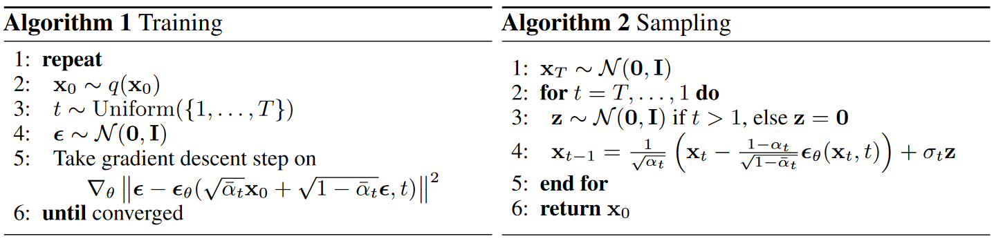
Empirically, Ho. et al. obtained better results in terms of sample quality (and simpler to implement) to train on the following variant of the variational bound:
$$ \begin{align} \label{eq:denosing_sm_simple} L_{\text{simple}}(\theta) &= \mathbb{E}_{t, \mathbf{x}_0, \mathbf{\epsilon}}\Big[ \Big|\Big| \mathbf{\epsilon} - \color{green}\mathbf{\epsilon}(\mathbf{x}_t, t) \color{black}\Big|\Big|^2\Big]; \quad t \sim U[1,T] \end{align} $$
Summary
To summarize, we can train the reverse process mean function approximator \(\mathbf{\mu}_{\theta}\) to predict \(\tilde{\mu}_t\), or by modifying its parameterization, we can train it to predict \(\mathbf{\epsilon}\).
-
We start with a predefined forward process that evolves over a time interval $t\in[0,T]$, systematically converting input data, $\mathbf{x}_0$, into noise through a perturbation kernel $q(\mathbf{x}_t \vert \mathbf{x}_{t-1})$ using a noise schedule $\beta_t$.
$$ \begin{equation} q(\mathbf{x}_t \vert \mathbf{x}_{t-1}) = \mathcal{N}(\mathbf{x}_t; \sqrt{1 - \beta_t} \mathbf{x}_{t-1}, \beta_t\mathbf{I}); \quad q(\mathbf{x}_{0:T})= q(\mathbf{x}_0) \prod_{t=1}^T q(\mathbf{x}_t \vert \mathbf{x}_{t-1} ) \end{equation} $$
- It is analytically possible to know the distribution of \(\mathbf{x}_t\) given \(\mathbf{x}_0\) by repeated application of \(q(\mathbf{x}_t \vert \mathbf{x}_{t-1})\)
$$ \begin{aligned} q(\mathbf{x}_{t-1} \vert \mathbf{x}_t, \mathbf{x}_0) &= \mathcal{N}(\mathbf{x}_{t-1} ; \tilde{\mu}_t(\mathbf{x}_t,\mathbf{x}_0), \tilde{\beta}_t\mathbf{I})\\ \text{where } \tilde{\mu}_t(\mathbf{x}_t,\mathbf{x}_0) &:= \frac{\sqrt{\bar{\alpha}_{t-1}}\beta_t}{1 - \bar{\alpha}_t }\mathbf{x}_0 + \frac{\sqrt{\alpha_t}(1 - \bar{\alpha}_{t-1})}{1 - \bar{\alpha}_t }\mathbf{x}_t \text{ and } \tilde{\beta}_t :=\frac{1 - \bar{\alpha}_{t-1}}{1 - \bar{\alpha}_t }\beta_t \end{aligned} $$
-
Training is performed by minimizing the cross entropy \(H[q(\mathbf{x}_0),p_{\theta}(\mathbf{x}_0)]\) between the true underlaying distribution \(q(\mathbf{x}_0)\) and the model probability \(p_{\theta}(\mathbf{x}_0)\). The CE measures the average number of bits needed to identify an event drawn from the set if a coding scheme used for the set is optimized for an estimated probability distribution p, rather than the true distribution q.
(*) The nice property of this derivation is that now all KL divergences are comparisons between Gaussians, so they can be calculated in a Rao-Blackwellized fashion with closed form expressions instead of high variance Monte Carlo estimates
: -
When \(\beta_t\) is small the reverse process have the same functional form of the forwar process. Therefore, the diffusion model is a parameterized a Gaussian distribution \(p_\theta(\mathbf{x}_{t-1} \vert \mathbf{x}_t) = \mathcal{N}(\mathbf{x}_{t-1}; \mathbf{\mu}_\theta(\mathbf{x}_t, t), \mathbf{\Sigma}_\theta(\mathbf{x}_t, t))\).
$$ \begin{aligned} \text{where } \tilde{\mu}_t(\mathbf{x}_t,\mathbf{x}_0) &:= \frac{\sqrt{\bar{\alpha}_{t-1}}\beta_t}{1 - \bar{\alpha}_t }\mathbf{x}_0 + \frac{\sqrt{\alpha_t}(1 - \bar{\alpha}_{t-1})}{1 - \bar{\alpha}_t }\mathbf{x}_t \text{ and }\\ \mathbf{\Sigma}_\theta(\mathbf{x}_t, t)&= \sigma_t\mathbf{I} \text{ and } \sigma_t:=\tilde{\beta}_t=\frac{1 - \bar{\alpha}_{t-1}}{1 - \bar{\alpha}_t }\beta_t \end{aligned} $$
-
By substitution \(\mathbf{x}_0 = \frac{1}{\sqrt{\bar{\alpha}_t}}(\mathbf{x}_t - \sqrt{(1 - \bar{\alpha}_t)}\mathbf{z_t}) \), we can reexpress \(\tilde{\mu}_t(\mathbf{x}_t,\mathbf{x}_0)\), the forward mean posterior, as
$$ \begin{aligned} \tilde{\mu}_t(\mathbf{x}_t,\mathbf{x}_0) &= \color{blue} \frac{1}{\sqrt{\alpha_t}}\Big(\mathbf{x}_t - \frac{\beta_t}{\sqrt{1 - \bar{\alpha}_t}} \mathbf{z_t}\Big)\\ \end{aligned} $$
$$ \begin{aligned} L_\text{CE} &= \mathbb{E}_{q(\mathbf{x}_0)}\left[-\log p_\theta(\mathbf{x}_0)\right] \\ &= \mathbb{E}_{q(\mathbf{x}_0)}\left[ -\log \Big( \mathbb{E}_{q(\mathbf{x}_{1:T} \vert \mathbf{x}_0)} \left[p(\mathbf{x}_T) \prod^T_{t=1} \frac{p_\theta(\mathbf{x}_{t-1} \vert \mathbf{x}_t)}{q(\mathbf{x}_t\vert \mathbf{x}_{t-1})}\right] \Big)\right] \\ &\leq \mathbb{E}_{q(\mathbf{x}_0)}\left[ \mathbb{E}_{q(\mathbf{x}_{1:T} \vert \mathbf{x}_0)} \left[-\log \Big(p(\mathbf{x}_T) \prod^T_{t=1} \frac{p_\theta(\mathbf{x}_{t-1} \vert \mathbf{x}_t)}{q(\mathbf{x}_t\vert \mathbf{x}_{t-1})}\Big)\right] \right] \\ &\leq \mathbb{E}_{q(\mathbf{x}_{0:T})} \left[-\log \Big(p(\mathbf{x}_T) \prod^T_{t=1} \frac{p_\theta(\mathbf{x}_{t-1} \vert \mathbf{x}_t)}{q(\mathbf{x}_t\vert \mathbf{x}_{t-1})}\Big) \right] = \color{blue}\mathbb{E}_{q(\mathbf{x}_{0:T})}\Big[\log \frac{q(\mathbf{x}_{1:T} \vert \mathbf{x}_{0})}{p_\theta(\mathbf{x}_{0:T})} \Big] = L_\text{VLB}\\ &= \mathbb{E}_{q(\mathbf{x}_{0:T})} \left[-\log p(\mathbf{x}_T) - \log\prod^T_{t=1} \frac{p_\theta(\mathbf{x}_{t-1} \vert \mathbf{x}_t)}{q(\mathbf{x}_t\vert \mathbf{x}_{t-1})} \right] \\ &= \mathbb{E}_{q(\mathbf{x}_{0:T})} \left[-\log p(\mathbf{x}_T) - \sum^T_{t=1}\log \frac{p_\theta(\mathbf{x}_{t-1} \vert \mathbf{x}_t)}{q(\mathbf{x}_t\vert \mathbf{x}_{t-1})} \right]\\ &= \mathbb{E}_{q(\mathbf{x}_0)}\left[ \underbrace{\text{D}_{KL}(q(\mathbf{x}_T \vert \mathbf{x}_0)||p(\mathbf{x}_T))}_{L_T} + \sum^T_{t=2} \underbrace{\text{D}_{KL} (q(\mathbf{x}_{t-1} \vert \mathbf{x}_t, \mathbf{x}_0)||p_\theta(\mathbf{x}_{t-1} \vert \mathbf{x}_t))}_{L_{t-1}} - \underbrace{\log p_\theta(\mathbf{x}_0 \vert \mathbf{x}_1)}_{L_0} \right];\quad \text{Markov property + Bayes' rule (*).}\\ &=\mathbb{E}_{q(\mathbf{x}_0)}\left[\sum^T_{t=2} \underbrace{\text{D}_{KL} (q(\mathbf{x}_{t-1} \vert \mathbf{x}_t, \mathbf{x}_0)||p_\theta(\mathbf{x}_{t-1} \vert \mathbf{x}_t))}_{L_{t-1}} - \underbrace{\log p_\theta(\mathbf{x}_0 \vert \mathbf{x}_1)}_{L_0} \right]\\ &= \mathbb{E}_{q(\mathbf{x}_0)}\left[\sum^T_{t=2}\underbrace{\text{D}_{KL} (q(\mathbf{x}_{t-1} \vert \mathbf{x}_t, \mathbf{x}_0)||p_\theta(\mathbf{x}_{t-1} \vert \mathbf{x}_t))}_{L_{t-1}}\right] - \mathbb{E}_{q(\mathbf{x}_0)}\left[\underbrace{\log p_\theta(\mathbf{x}_0 \vert \mathbf{x}_1)}_{L_0} \right]\\ &=\mathbb{E}_{q(\mathbf{x}_0)}\left[\sum^T_{t=2}\underbrace{\mathbb{E}_{q(\mathbf{x}_{t-1} \vert \mathbf{x}_t, \mathbf{x}_0)}\Big[\log \frac{q(\mathbf{x}_{t-1} \vert \mathbf{x}_t, \mathbf{x}_0)}{p_\theta(\mathbf{x}_{t-1} \vert \mathbf{x}_t)}}_{L_{t-1}} \Big]\right]\\ &=\mathbb{E}_{q(\mathbf{x}_0)}\left[\sum^T_{t=2}\mathbb{E}_{q(\mathbf{x}_{t-1} \vert \mathbf{x}_t, \mathbf{x}_0)}\Big[\log \frac{\mathcal{N}(\mathbf{x}_{t-1} ; \tilde{\mu}_t(\mathbf{x}_t,\mathbf{x}_0), \tilde{\beta}_t\mathbf{I})}{\mathcal{N}(\mathbf{x}_{t-1}; \mathbf{\mu}_\theta(\mathbf{x}_t, t), \sigma_t^2\mathbf{I})} \Big]\right]\\ &=\mathbb{E}_{q(\mathbf{x}_0)}\left[\sum^T_{t=2}\mathbb{E}_{q(\mathbf{x}_{t-1} \vert \mathbf{x}_t, \mathbf{x}_0)}\Big[LLR (\mathbf{x}_{t-1})\Big]\right]\\ &= \mathbb{E}_{q(\mathbf{x}_0)}\left[\sum^T_{t=2} \mathbb{E}_{q(\mathbf{x}_{t-1} \vert \mathbf{x}_t, \mathbf{x}_0)}\Big[\frac{1}{2\sigma_t^2}||\tilde{\mu}_t(\mathbf{x}_t,\mathbf{x}_0)-\mu_{\theta}(\mathbf{x}_t,t)||^2\Big]\right]\\ &= \mathbb{E}_{q(\mathbf{x}_0)}\left[\sum^T_{t=2} \mathbb{E}_{\mathbf{x}_0, \mathbf{\epsilon}}\Big[\frac{1}{2\sigma_t^2}\Big|\Big|\tilde{\mu}_t\Big(\mathbf{x}_t(\mathbf{x}_0, \mathbf{\epsilon}),\frac{1}{\sqrt{\bar{\alpha}_t}}(\mathbf{x}_t(\mathbf{x}_0, \mathbf{\epsilon})- \sqrt{1 - \bar{\alpha}_t}\mathbf{\epsilon})\Big)-\mu_{\theta}(\mathbf{x}_t(\mathbf{x}_0, \mathbf{\epsilon}),t)\Big|\Big|^2\Big]\right] \\ &= \mathbb{E}_{q(\mathbf{x}_0)}\left[\sum^T_{t=2} \mathbb{E}_{\mathbf{x}_0, \mathbf{\epsilon}}\Big[\frac{1}{2\sigma_t^2}\Big|\Big|\color{blue}\frac{ 1}{\sqrt{\alpha}_t} \Big(\mathbf{x}_t(\mathbf{x}_0, \mathbf{\epsilon}) \color{red}-\frac{\beta_t}{\sqrt{1 - \bar{\alpha}_t}} \mathbf{\epsilon}\Big)\color{black}-\mu_{\theta}(\mathbf{x}_t(\mathbf{x}_0, \mathbf{\epsilon}),t)\Big|\Big|^2\Big]\right]\\ &= \mathbb{E}_{q(\mathbf{x}_0)}\left[\sum^T_{t=2} \mathbb{E}_{\mathbf{x}_0, \mathbf{\epsilon}}\Big[\frac{1}{2\sigma_t^2}\Big|\Big|\color{blue}\frac{ 1}{\sqrt{\alpha}_t} \Big(\mathbf{x}_t \color{red}-\frac{\beta_t}{\sqrt{1 - \bar{\alpha}_t}} \mathbf{\epsilon}\Big)\color{black}-\color{blue}\frac{ 1}{\sqrt{\alpha}_t} \Big(\mathbf{x}_t\color{red}-\frac{\beta_t}{\sqrt{1 - \bar{\alpha}_t}} \color{green}\mathbf{\epsilon}_{\theta}(\mathbf{x}_t, t)\color{black}\Big)\Big|\Big|^2\Big]\right]; \text{ Parameterization}\\ &= \mathbb{E}_{q(\mathbf{x}_0)}\left[\sum^T_{t=2} \mathbb{E}_{\mathbf{x}_0, \mathbf{\epsilon}}\Big[\frac{1}{2\sigma_t^2}\Big|\Big|\color{blue}-\frac{ 1}{\sqrt{\alpha}_t}\color{red}\frac{\beta_t}{\sqrt{1 - \bar{\alpha}_t}} \color{black}(\mathbf{\epsilon}\color{red}-\color{green}\mathbf{\epsilon}_{\theta}(\mathbf{x}_t, t)\color{black})\Big|\Big|^2\Big]\right]\\ &= \mathbb{E}_{q(\mathbf{x}_0)}\left[\sum^T_{t=2} \mathbb{E}_{\mathbf{x}_0, \mathbf{\epsilon}}\Big[ \frac{\beta_t^2}{2\sigma_t^2\alpha_t(1 - \bar{\alpha}_t)}\Big|\Big| \mathbf{\epsilon} - \color{green}\mathbf{\epsilon}_{\theta}(\mathbf{x}_t, t) \color{black}\Big|\Big|^2\Big]\right]\\ &= \mathbb{E}_{q(\mathbf{x}_0)}\left[\mathbb{E}_{t, \mathbf{x}_0, \mathbf{\epsilon}}\Big[ \Big|\Big| \mathbf{\epsilon} - \color{green}\mathbf{\epsilon}(\mathbf{x}_t, t) \color{black}\Big|\Big|^2\Big]\right]=L_{\text{simple}}(\theta); \quad t \sim U[1,T] \end{aligned} $$
Interpretation The variational lower bound objective tell us that what we have to minimize is the log-likelihood ration of the forward trajectory wrt the reverse estimated trajectory average over forward trajectories. If \(LLR = 1 \rightarrow L_\text{VLB}=0\). This objective function aims to obtain a model that in average describe the same forward trajectories but in reverse.
Continuous diffusion Models
Applications
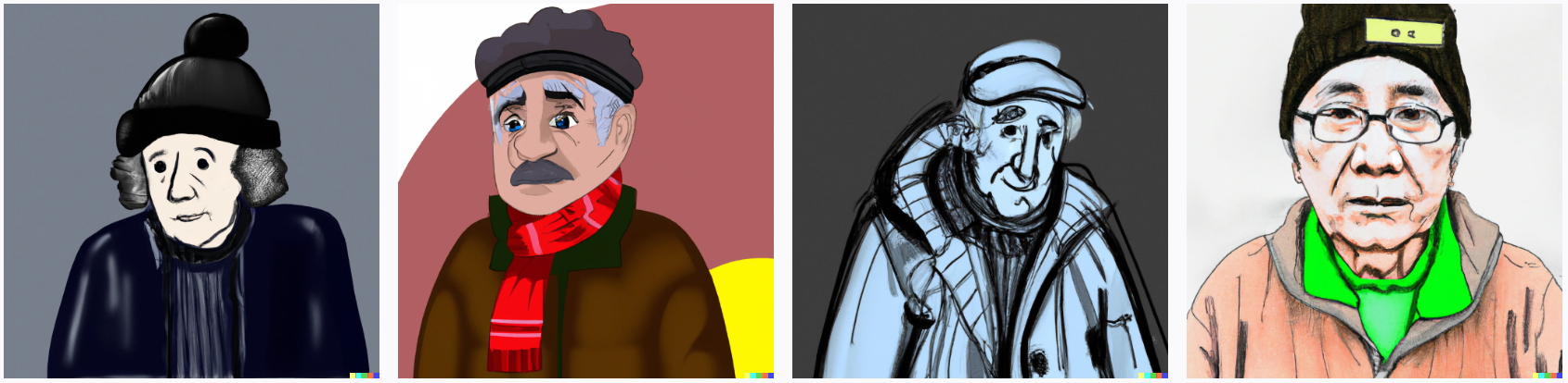
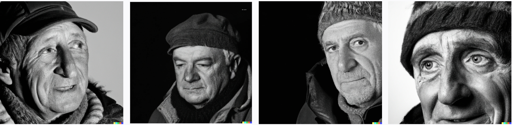
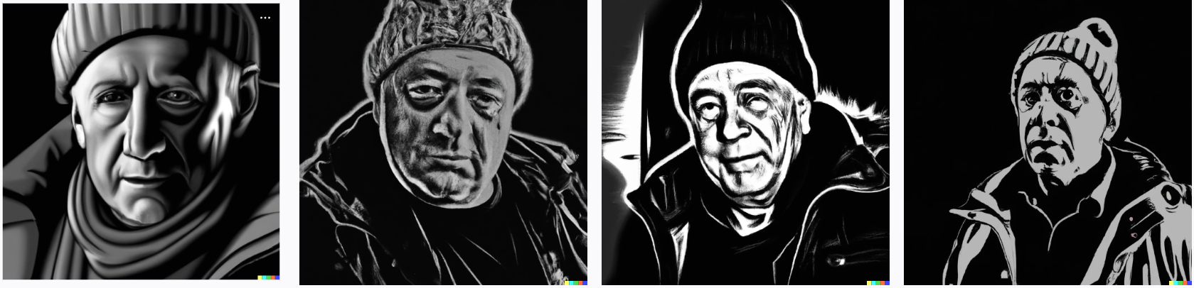
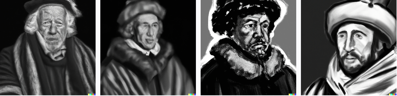
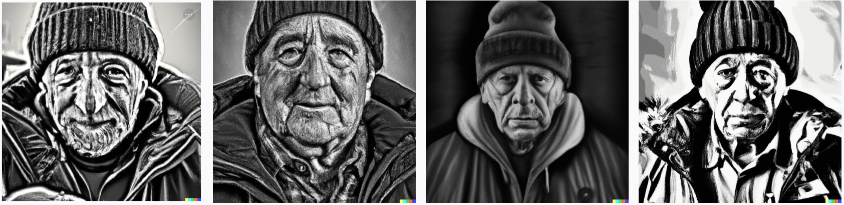
Generative models can be used for several applications. One recent remarkable application is DALL-E 2, a new AI system that can create realistic images and art from a description in natural language. DALL-E 2 uses diffusion models to produce high-quality image samples. For more details about DALL-E 2 see the scientific paper Text-Conditional Image Generation with CLIP Latents
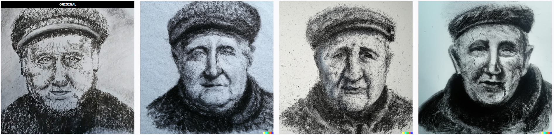
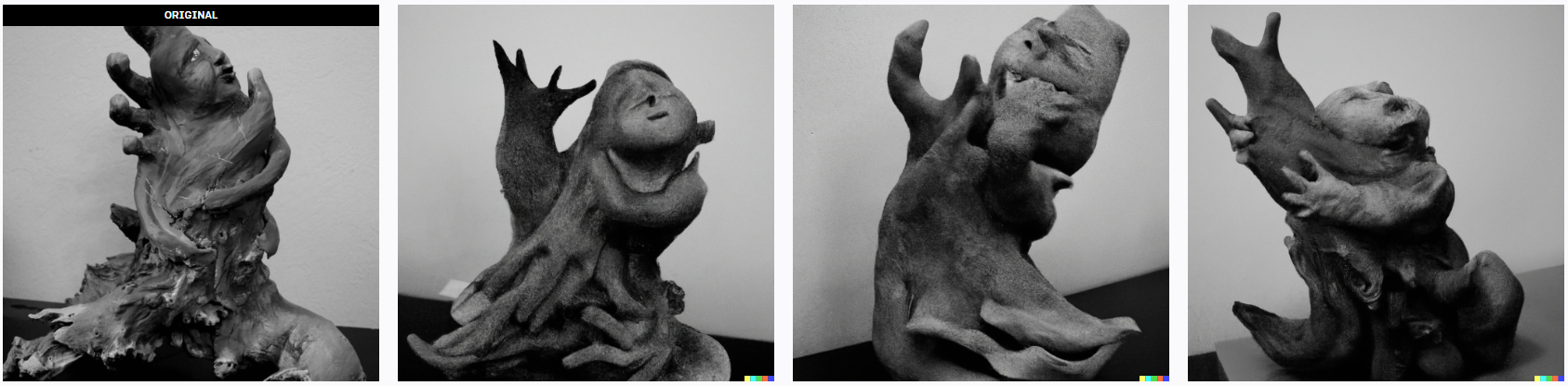
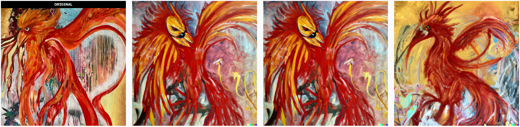
You can also ask DALL-E 2 to generate an image given a text. Let's try to recreate the original art from above with DALL-E 2. Figure 4 shows several queries that attempt to recreate the drawing of the older man from above. However, as you can see, DALL-E 2 requires an accurate description to match what you have in mind, the more specific the query. The more information DALL-E 2 has to create what you might expect! Yet, you can as well get surprised with new ideas!